In certain circumstances, you will run into situations where the issue
limiting the timesteps is the mysterious newton_iters. To demonstrate this, I'll be using the wd2 test case from MESA version
7624 with a few minor changes:
Lowered accretion rate to 5e-8.
Shut off super-Eddington wind.
These are sufficient to make things really difficult for the solver when
the first nova goes off and the envelope expands to large sizes.
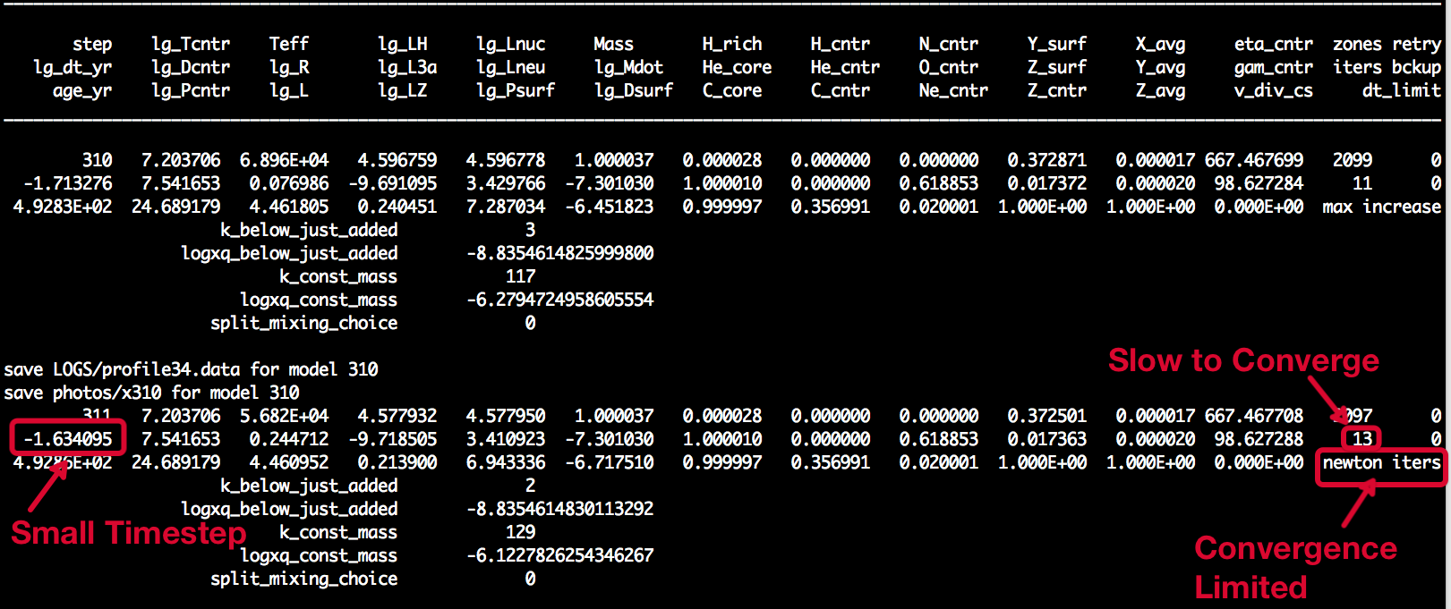
You don't want to be seeing this. Terminal output from the example case when
the solver starts struggling.
The simple solution would be to raise the maximum number of iterations
allowed. In controls.defaults, one finds
! limits based on iterations required by various solvers and op-splitting!### newton_iterations_limit! If newton solve uses more `newton_iterations` than this, reduce the next timestep.newton_iterations_limit=7
We could simply add something like newton_iterations_limit = 7
to our inlist to "solve" the problem. However, this doesn't really address the
problem that MESA is struggling to converge because of your model (there are
times for adjusting the above setting, but I'm not overly familiar with
them). Rather, there is probably (hopefully?) something you can do to just
make the number of iterations required to go down.
Finding out more information
There are inlist commands available to you that can tell you more about the
struggle that the solver is going through. They are stored in the aptly-named
debugging_stuff_for_inlists which lives in the test suite directory.
The full list of commands there is
! FOR DEBUGGING!report_hydro_solver_progress = .true. ! set true to see info about newton iterations!report_ierr = .true. ! if true, produce terminal output when have some internal error!hydro_show_correction_info = .true.!max_years_for_timestep = 3.67628942044319d-05!report_why_dt_limits = .true.!report_all_dt_limits = .true.!report_hydro_dt_info = .true.!show_mesh_changes = .true.!mesh_dump_call_number = 5189!okay_to_remesh = .false.!trace_evolve = .true.! hydro debugging!hydro_check_everything = .true.!hydro_inspectB_flag = .true.!hydro_numerical_jacobian = .true.!hydro_save_numjac_plot_data = .true.!hydro_dump_call_number = 195!hydro_dump_iter_number = 5!trace_newton_bcyclic_solve_input = .true. ! input is "B" j k iter B(j,k)!trace_newton_bcyclic_solve_output = .true. ! output is "X" j k iter X(j,k)!trace_newton_bcyclic_steplo = 1 ! 1st model number to trace!trace_newton_bcyclic_stephi = 1 ! last model number to trace!trace_newton_bcyclic_iterlo = 2 ! 1st newton iter to trace!trace_newton_bcyclic_iterhi = 2 ! last newton iter to trace!trace_newton_bcyclic_nzlo = 1 ! 1st cell to trace!trace_newton_bcyclic_nzhi = 10000 ! last cell to trace; if < 0, then use nz as nzhi!trace_newton_bcyclic_jlo = 1 ! 1st var to trace!trace_newton_bcyclic_jhi = 100 ! last var to trace; if < 0, then use nvar as jhi!trace_k = 0
I personally don't know what most of these do, but we can get a lot done
with just three of these commands. First, you should copy all of the contents of
debugging_stuff_for_inlists to the controls section
of your inlist. Then, you should uncomment the first line:
report_hydro_solver_progress=.true.! set true to see info about newton iterations
Running your model again will now produce a lot more output,
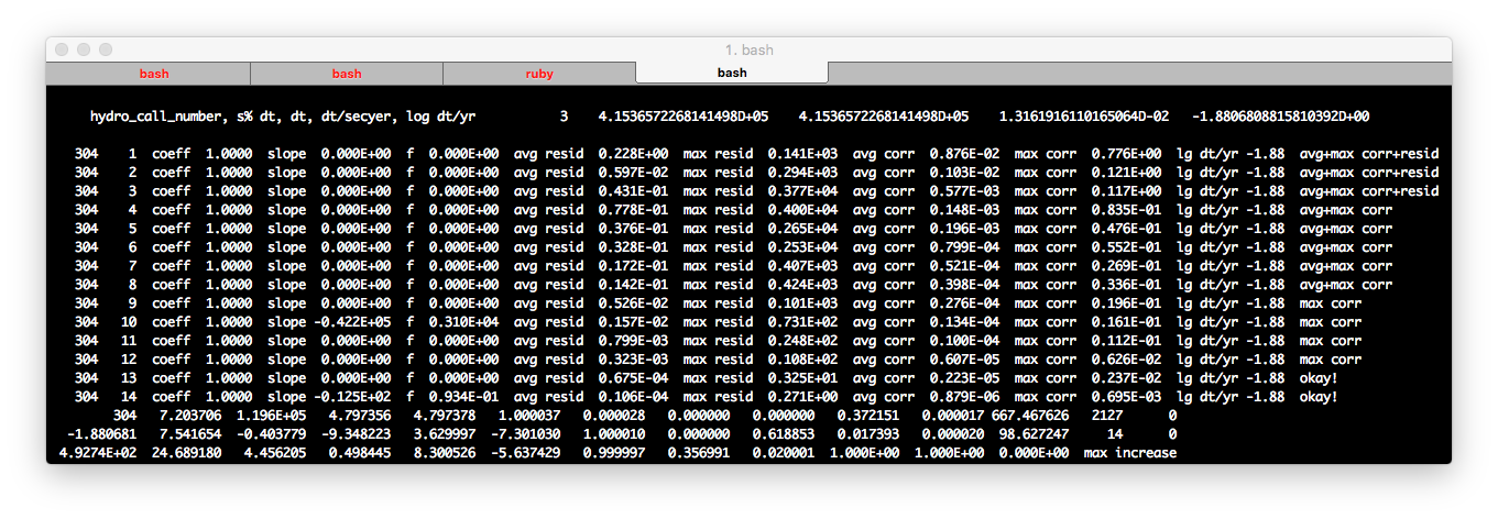
giving information about each and every call to the solver:
Terminal output when displaying hydro solver progress.
The above screenshot shows the output after turning on the reporting of
hydro solver information. You can see there is an initial line that gives
some general information about the call to the solver:
In particular, the value for hydro_call_number will be of
interest to us (in this case it's 1). Then, there is a series six lines that
give step by step summaries of what the solver did. The last column is the
simplest to understand. It tells us that for the first four steps, the solution
was rejected because the correction from the last guess was too deviant. In
those cases, the average correction over the whole model was too large, and the
largest correction in any one location was also too large. By the fourth
iteration, the neither of these corrections were too large, and after being
"fine" on the fifth iteration, it decided the solution was good enough.
You'll note that in the timestep, the number of steps (6) is also recorded in
the normal terminal output (second to last column, second row). Normally this is
the only information you get about the hydro solver unless a retry or backup
is required.
Now that we can track the progress of the solver, we should get to a time
when things are really bad:
Ouch! Fourteen steps is way over our default tolerance of 7. You can bet
the next step will have a reduced timestep with a reason of "newton_iters". We
see now that the last problem to "give" is the max coorection (steps 9-12). So
there's probably a troublesome location within the star that is the real issue
here, rather than generally poor temporal or spatial resolution. Now let's
really dig into the guts!
Pinpointing the Problem
Now we make a directory in our work directory called "plot_data" and another
directory inside of that one called "solve_logs". We're going to instruct MESA
to dump all the solver data into this directory (solve_logs) for the one
problematic timestep.
To do this, we uncomment two more lines of the debugging material we added
to our inlist. The first is hydro_inspectB_flag = .true..
B is the name of the vector of corrections in the hydro solver, so
we are telling MESA to actually look at that stuff. The second line is
hydro_dump_call_number = 195. The number 195 here is really just
random. We'll be replacing it with the hydro_call_number from
the timestep we want to investigate. The reason we can't use a model number is
because due to retries and backups, any given timestep could have an arbitrary
number of calls to the hydro solver, so the solver call number is a unique
identifier. In this case, for the model shown above, we'll want to put in a
value of 3 (see the first line before all of the iterations).
Now if we rerun the model, it will crash once it has completed it's call to
the hydro solver at the call number we specified. Our new plot_data/solve_logs
directory will be chock full of data files.
These new files aren't as user-friendly as the profiles and history files
you're used to. The data for most files is two-dimensional, giving values of
various quantities (like the log of the density, or the corrections thereof)
at each grid point and at each iteration. So for a model with
N zones and M iterations, each of these data files will
have N × M entries. They are not arranged in a grid,
so using the data requires a little manipulation.
The Tioga Way
The simplest solution to this problem is to use Bill Paxton's nifty Tioga
script solve_log.rb found in many test suite cases (for example,
wd2 has it in its plotters directory as of version 7624).
Dropping this file in your plot_data directory and replacing the various
instances of "../../../.." with an explicit path to your $MESA_DIR
gives you quick access to some informative plots. For instance, running
tioga solve_log -s 0
produces a nice image plot of the correction to density as a function of the
iteration (y-axis) and the grid point (x-axis), as shown below.
Image plot of corrections to the log of density as made by Bill Paxton's Tioga
script. Bright colors indicate large corrections.
Varying the values of first_row and last_row let
you hone in on particular iterations, and changing first_col and
last_col lets you hone in on particular grid points (this is the
useful one). We'll get to interpreting the data in a moment, but first...
The Python Way
Word on the street is that the cool kids these days use Python to make
plots, so I coded up a file that emulates what Bill Paxton's tioga scripts do.
You can find a version of it here (requires
numpy and matplotlib). An updated (and possibly better) version should also be
available on MesaStar.org. You can either run
it interactively in iPython (or just the regular python shell if that's your
thing) or run it straight from the shell via python solve_log.py
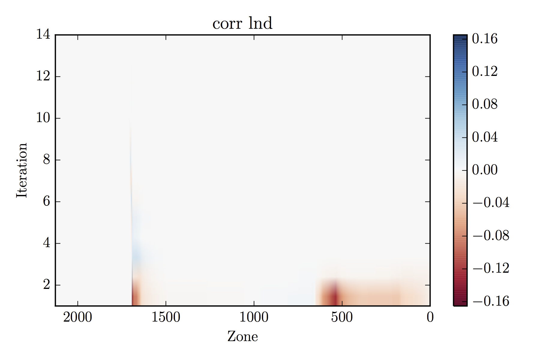
which will produce the default plot, which shows the corrections in the log of
the density over all grid points and all iterations, making a pdf called
corr_lnd.pdf:
Image plot of corrections to the log of density as made by my Python
script. Bright colors indicate large corrections.
Or you could code your own thing up.
Anyway, it looks like there's a problem that persists for many iterations
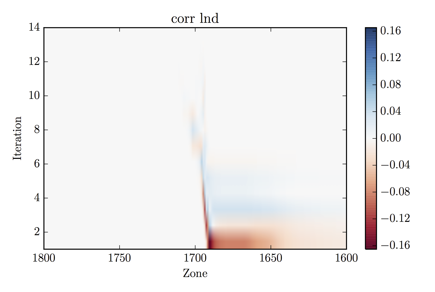
near zone 1700. Let's adjust the x-axis to zoom in on that issue. To do this,
we alter the first_col and last_col to 1600 and 1800,
respectively (in the Tioga case)
Zoom of previous plot... yep, the issue around point 1700 is definitly the
cause of the problem.
So indeed, it is this area that is causing convergence difficulties. Let's
look at what might be causing this.
Comparing to the model
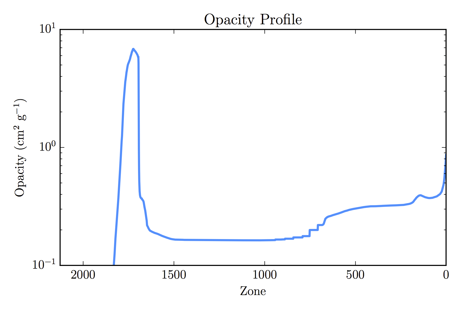
My suspicion is that due to the large envelope, opacity problems may be the
source of the issue, so I went back and re-ran things with a maximum model
number of 304, being sure to save the last profile. The opacity then looks like
Well lookee here... A spike around zone 1700!
So it looks like the convergence errors are related to the extreme bump in
opacity.
Solving the Problem
Now that we know something about the problem, we might look at related
quantities (perhaps the opacity bump causes a density inversion? Maybe there
are supersonic velocities here? Is it even convectively unstable? What does
the pressure profile look like?).
When you identify what is physically going on, the first question is "Do I
even care about this region of the star?" If the answer is no, the easiest
solution is to cut this part out. If it's in the core, try removing the
core from the model (like in the ccsn test case or the neutron star test
cases). If it's near the surface, you might move the outer boundary condition
inwards, likely using the tau_factor controls.
If however, you do care about what's going on in the troublesome
region, you'll need to think hard about a solution that eases the numerical
convergence without doing an unaccepatable amount of damage to the
believability of the model. For this case, turning on MLT++ (via okay_to_reduce_gradT_excess = .true. and friends) is probably a
good first step towards easing the convergence. There is, however no
silver bullet.